NCAA Tournament 2017 Model
Take two on building a model to produce a decent bracket for the 2017 NCAA Men’s Basketball Tournament.
The madness of March is here, and I’m once again trying to figure out this madness with a sound statistical model for the 2017 NCAA Men’s Basketball Tournament. Despite my bracket’s terrible 15th percentile performance from last year, I’m still determined to make a model that excels in the bracket competition. Conceptually, I think a model is well positioned to compete in this competition due to the plethora of data points. This tournament (and the accompanying regular seasons) has been going on for years and has been well documented in terms of stats and metrics. With so many variables and trials, a model should be able to find patterns that can predict the outcome of tournament games. A big challenge to the model, however, is the unforgiving single elimination nature of the NCAA tournament, where a single game can break brackets. Due to the large impact this randomness has on a bracket’s performance, it’ll be difficult to discern long-term performance from short-term results. To succeed, the model will have to discern signal from noise and upset from fluke.
In this project, I will go through the following steps to produce a bracket for the 2017 tournament:
- Collect data
- Explore variables
- Explore different types of model structures
- Results of the bracket
Collect data
All the data for this model comes from Kaggle’s 2017 NCAA Tournament competition. The dataset includes regular season and tournament data from 1985 to 2016. The data includes basic box score metrics, such as shot attempts, rebounds, assists, steals, etc. Unfortunately, the data does not contain any advanced metrics or rankings, such as RPI, BPI, and AP rankings.
Explore variables
To determine which simple and derived variables to use, I first brainstormed which factors would have the biggest impact on tournament outcomes. The list included:
- Pace (Number of Possessions and Consistency of this Pace)
- Offensive and Defensive Efficiency per Possession
- Winning Percentage and Strength of Regular Season Schedule
- Success on the Road
- 3 Point Percentage on Offensive and Defense
- Close Game Performance
Using the regular season data from Kaggle, I created metrics that are proxies to each of these features. The exact variable definitions as well as their distribution can be found here. Next, I looked at the relationship between these variables and the margin of victory for tournament games. The full results can be found here.
The top two variables were strength of schedule and regular season winning percentage:
- Strength of Schedule (SOS): teams with harder strength of schedules generally had higher margins of victories. Winning teams had a 0.34 correlation between their SOS and margin of victory, while losing teams have a -0.40 correlation between their SOS and margin of victory.
- Regular Season Winning Percentage: there was a 0.32 correlation for the winning team’s winning percentage and a -0.34 correlation for the losing team’s winning percentage.
Most surprising was that my derived variable, close game performance, had a correlations in the opposite direction than I hypothesized. This variable was meant to represent a team’s performance in the clutch. I split a team’s games into two categories: close games and not close games. Close games were defined as those that went into OT or were decided by 5 points or less. Using this partition of regular season games, I calculated the difference in winning percentage with this formula:
Close Game Performance = (Winning Percentage of Close Games) - (Winning Percentage of Not Close Games)
My hypothesis was that teams that performed well in these close games would also perform well in future close, competitive games, such as those in the tournament. However, my hypothesis appeared to be false. There was a negative correlation between this metric and the margin of victory, suggesting that teams that relatively did better in closer regular season games did worse in tournament games. For the winning team, the correlation was -0.14, and for the losing team, the correlation was 0.12. Though I did not dig further into why this hypothesis was incorrect, I think this variable warrants more analysis, especially in how it interacts with other variables, such as the difference in opponent strength of schedule for close and not close games.
Finally, I decided to consolidate the other variables in an effort to describe team playing styles. My hypothesis was that each team has a preferred playing style and that each of these playing styles has advantages and disadvantages over other types of styles. To figure out these playing styles, I used three variables, offensive efficiency, defensive efficiency, and pace variables, to form clusters using a K-Means model. Here are the results of running the model with 2, 3, and 4 clusters.
2 Clusters
3 Clusters
4 Clusters
Based on these plots, I determined that 3 clusters made most sense. Based on the graphs, the 4 cluster model appeared to have too many groups, while the 2 cluster model seemed a bit too simplistic. The 3 cluster model was a nice compromise between simplicity and having distinct groups. When segmenting teams by this 3 cluster K-means model, I found these differences in margin of victory:
| Cluster 1 | Cluster 2 | Cluster 3 | ||||
| Cluster 1 | 0.44 | |||||
| Cluster 2 | 4.08 | -0.31 | ||||
| Cluster 3 | 7.05 | 2.07 | 1.30 |
There are some large swings in margin of victory among different cluster matchups, making me feel comfortable with this selection of clusters.
Explore model types
Now that I chose my set of variables, I next decided which model to use. Given that the target variable could be either a category (i.e. win vs lose) or a quantity (i.e. margin of victory), I evaluated model types in both classification and regression families:
- Ridge Regression
- Gradient Boosting Model
- Logistic Regression
- Support Vector Machine
Judging the performance of these models proved to be tricky as my objective wasn’t exactly the traditional objectives of maximizing classification accuracy or minimizing prediction error. My objective was to see which model produced the bracket with the most points. This meant that not all games mattered equally, so taking the average of classification accuracies or of squared errors would not be sufficient. I ended up making my own metric to evaluate success of these models:
Tournament points = (correct 1st round outcomes)*2^0 + (correct 2nd round outcomes)*2^1 + (correct 3rd round outcomes)*2^2 + (correct 4th round outcomes)*2^3 + (correct 5th round outcomes)*2^4 + (correct 6th round outcomes)*2^5
After running each of these models with the same inputs variables and cross-validating against their respective default scores (MSE for first two models and accuracy for last two), I obtained the two best models:
| Model Type | Tournament Score | |
| Ridge Regression | 82.5 | |
| Logistic Regression | 86.2 |
With these results, I decided to use logistic regression to make predictions for my bracket.
Results of the Bracket
The bracket did okay. In ESPN’s Bracket Challenge, it picked up 730 points (equivalent to 73 points in the tournament score mentioned above) and was in the 59th percentile. Looking at the round by round performance, the bracket started strong, but struggled immensely after the Sweet 16:
| Round of 64 | 250/320 | |
| Round of 32 | 240/320 | |
| Sweet 16 | 160/320 | |
| Elite Eight | 80/320 | |
| Final Four | 0/320 | |
| Championship | 0/320 |
Here’s the full bracket: 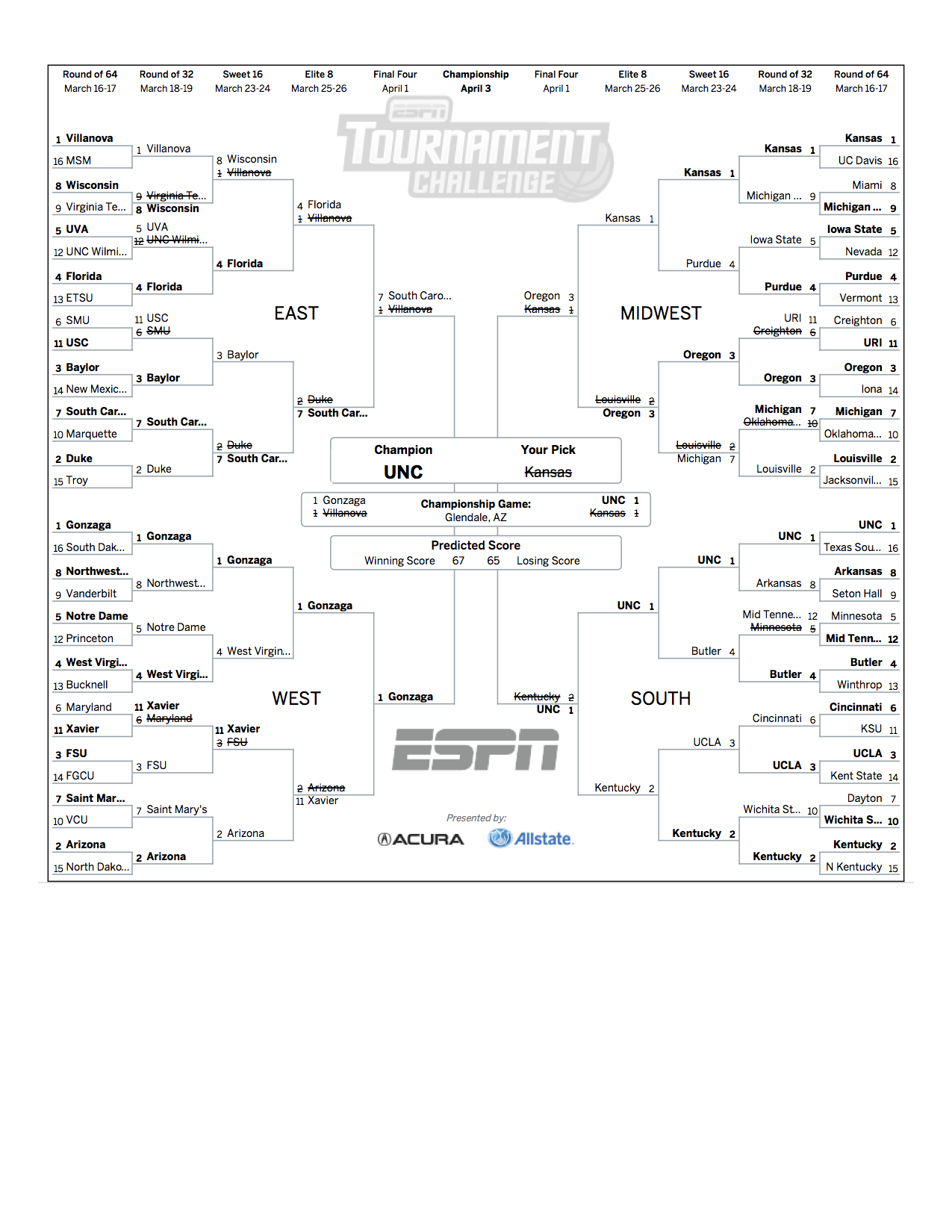
Next Steps
First off, this attempt was a relative success compared to my attempt last year. My bracket in 2016 placed in the 15th percentile, while this bracket in 2017 moved up to the 59th percentile. Though I made a lot of changes to my data, features, and modeling methodology, I’d hypothesize the biggest contributing factor to this improvement was how I trained the models. In 2016, I used regular season outcomes to train and evaluate my models. This year, I used past tournament outcomes to train my models and evaluated them on their simulated point performance. Truing the evaluation metric to tournament points gave me a much better idea of each model’s performance and likely resulted in better model building decisions.
Looking forward, I think there is still a lot of room for improvement and that the 59th percentile is nowhere near the ceiling for a model-based bracket.
Based on the results of this model and of last year’s model, I think getting more data would have the most impactful improvement to my model. This model relied upon traditional basketball metrics summarized at the game level. It lacked two other categories of variables: advanced statistics and human rankings. For advanced statistics, I think having statistics incorporating player movement data would give the model a much better sense of a team’s style of play, including team and player weaknesses and strengths. Human rankings, such as AP polls, could help the model capture characteristics that we haven’t figured out how to describe in data yet. Given that the NCAA tournament selection committee incorporates both advanced statistics and human rankings into its decisions, including these variables will likely improve prediction power.